DriftRecon: One-Step Medical Image Reconstruction with Nullspace Drifting

A single-pass generative reconstructor for sparse-view CT and accelerated MRI that is data-consistent by construction and has a guidance knob for trading fidelity against realism.

Notes on DriftRecon (arXiv:2610.38953): guidance-coupled nullspace drifting for one-step medical image reconstruction in sparse-view CT and accelerated MRI.

← Research notes

Paper: Guidance-Coupled Nullspace Drifting for One-Step Medical Image Reconstruction (arXiv:2610.38953, eess.IV) Authors: M. Tuna Alatan, Agah Server Tapan, Şaban Öztürk, Muhammad Usama Mirza, Bilal Kabas, Ge Wang, Tolga Çukur

TL;DR. DriftRecon is a generative reconstructor that produces an image in one forward pass. Training and generation are confined to the nullspace of the imaging operator, so every output agrees exactly with the acquired measurements and no post-hoc data-consistency step is needed. A guidance parameter \alpha trades fidelity for realism at inference time. A guidance-dependent temperature schedule limits how much fidelity is lost as \alpha grows. On sparse-view CT and accelerated MRI it beats physics-driven unrolled networks, few-step diffusion/flow methods, and recent drifting models.

Why one-step generative reconstruction?

Undersampled acquisitions (fewer CT projection views, skipped MRI phase-encode lines) give an ill-posed inverse problem

y = A x^\star,

where A is the imaging operator, y the measurements, and x^\star the image we want. Generative priors (diffusion, flow matching) produce realistic texture where regression-trained networks oversmooth. They usually need many network evaluations, though, and that cost is hard to justify clinically.

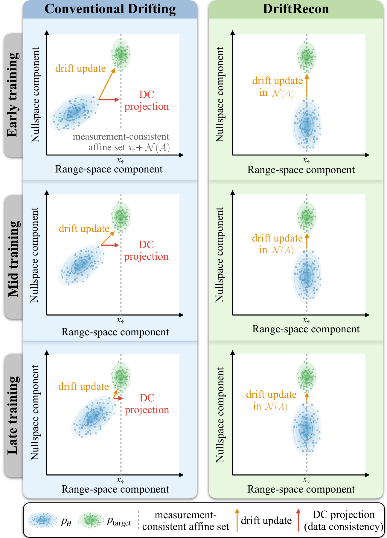
Drifting models offer a way around this. They do the iterative distribution matching during training: a kernel-based attraction–repulsion field pulls generated samples toward real data, and the generator learns to regress onto that moving target. At test time one evaluation is enough. Earlier drifting methods for medical imaging (RDDM, SA-RDM) apply the drift in the full image space. Part of each update then moves components that the measurements already determine, and a final data-consistency projection throws that part away.

Range–nullspace view

With the pseudoinverse A^\dagger, every image consistent with y lives on an affine set:

x^\star = \underbrace{A^\dagger y}_{x_\dagger} \;+\; \underbrace{(I - A^\dagger A)\,x^\star}_{z^\star \,\in\, \mathcal{N}(A)}, \qquad P_{\mathcal{N}} = I - A^\dagger A.

The anchor x_\dagger is fixed by the data. The only thing a reconstructor needs to infer is the nullspace component z^\star: the part of the image the scanner did not see.

Figure 1: Conventional drifting (left) moves samples in directions that include range-space components, which a data-consistency projection must then undo. DriftRecon (right) keeps the anchor x_\dagger fixed and confines generation and drift to \mathcal{N}(A), so A\hat x = y holds throughout training.

Method

Nullspace drifting

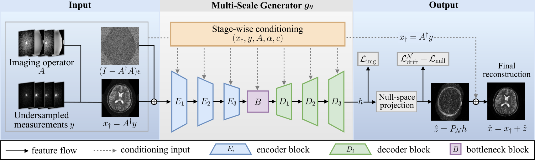
DriftRecon draws noise, projects it onto the nullspace, and runs it through a generator g_\theta conditioned on the anchor, the operator, the measurements, and the guidance strength. The output is projected back onto the nullspace:

\varepsilon^{\mathcal N} = \sigma P_{\mathcal N}\varepsilon, \qquad \hat z = P_{\mathcal N}\, g_\theta(\varepsilon^{\mathcal N}, x_\dagger, A, y, \alpha), \qquad \hat x = x_\dagger + \hat z.

Since A P_{\mathcal N} = 0, we get A\hat x = y exactly, for every sample, at every point in training.

The drift field is also built entirely in \mathcal N(A). The positive is the true nullspace component z^\star. The negatives are a second generated sample, plus nullspace components of other images in the batch (mismatched reals). Every input lies in the nullspace, so the drift does too. The generator is trained with a stop-gradient regression

\mathcal L_{\text{drift}} = \big\| \hat z - \mathrm{sg}(\hat z + V^{\mathcal N}) \big\|_2^2,

applied over the subbands of a multilevel Haar wavelet decomposition (for CT), with small auxiliary image- and nullspace-domain losses.

Physics-conditioned multiscale generator

The generator is a four-level convolutional encoder–decoder. Following RAM, it injects measurement conditioning inside every residual block, so the network sees A and y at every resolution and not only at the input or output. In the ablation below, removing this conditioning is one of the most damaging changes.

Figure 2: Generator architecture. Nullspace-projected noise and x_\dagger enter a multiscale network that is conditioned on A, y and \alpha throughout. The output is projected onto \mathcal N(A) and added to the anchor in a single forward pass.

Guidance and a temperature schedule to go with it

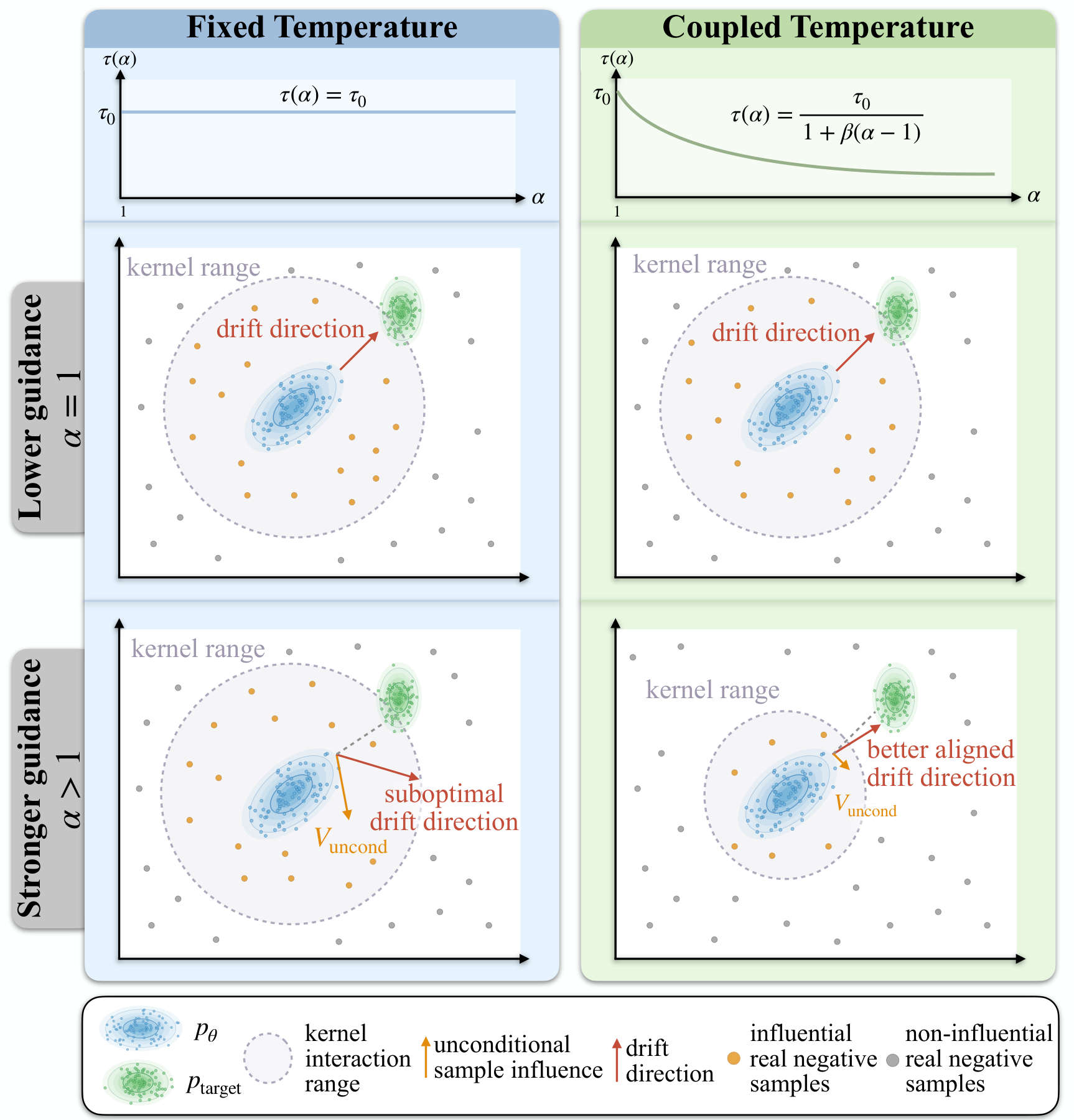
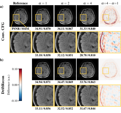
Guidance in drifting models works by mixing mismatched real images into the negative set. With weight 1 - 1/\alpha, the generator is pushed away from “generic” anatomy and toward the specific target, analogous to classifier-free guidance. \alpha = 1 is purely conditional. Larger \alpha increases realism, but with a fixed kernel temperature \tau it also lets distant mismatched samples distort the drift, and fidelity drops quickly.

We look at the relative weight a mismatched negative receives as \alpha changes and require the guidance-weighted mass near the decision boundary to stay constant. That condition gives a simple closed form:

\tau(\alpha) = \frac{\tau_0}{1 + \beta(\alpha - 1)}.

Here \tau_0 is the temperature at \alpha = 1, and \beta = 0 recovers ordinary fixed-temperature drifting. Stronger guidance makes the kernel more local, so supervision stays focused on nearby samples. The single knob \alpha now controls both the fidelity–realism balance and the locality of the drift.

Figure 3: Fixed-temperature drifting versus the guidance-coupled schedule. At \alpha=1 they coincide. For \alpha>1, the shrinking temperature keeps far-away mismatched samples from dominating the drift.

Experiments

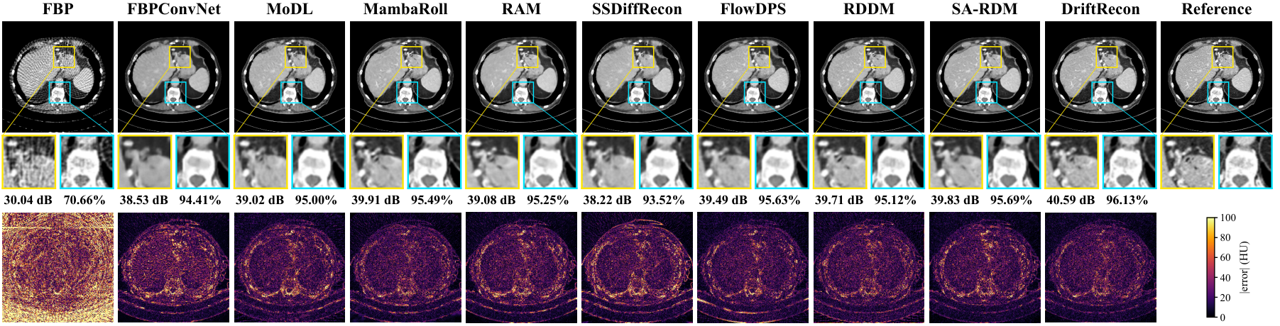
• Sparse-view CT. NIH–AAPM–Mayo Low-Dose CT Grand Challenge (abdominal), parallel-beam geometry, R = 6 and R = 12.
• Accelerated MRI. M4Raw low-field (0.3 T) multicoil brain MRI (T1w, T2w, FLAIR), 2D variable-density masks, R = 4 and R = 8.
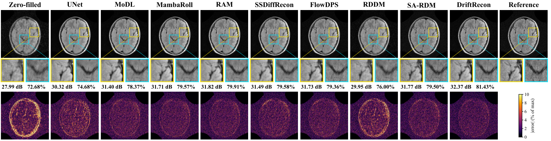
• Baselines. Data-driven (FBPConvNet / UNet). Physics-driven unrolled (MoDL, MambaRoll, RAM). Few-step generative with five steps (SSDiffRecon, FlowDPS). One-step drifting (RDDM, SA-RDM).

Results

Averaged across acceleration rates (SSIM in %, LPIPS ×100), best competitor in each column versus DriftRecon at \alpha = 1:

Task	Metric	Best competitor	DriftRecon
CT	PSNR ↑	39.31 (MambaRoll)	39.83
CT	SSIM ↑	94.98 (FlowDPS)	95.73
CT	LPIPS ↓	2.88 (RDDM)	1.96
CT	FID ↓	57.12 (RDDM)	37.45
MRI	PSNR ↑	30.95 (RAM)	31.37
MRI	SSIM ↑	80.66 (SA-RDM)	82.06
MRI	LPIPS ↓	8.22 (FlowDPS, SA-RDM)	6.61
MRI	FID ↓	11.80 (FlowDPS)	8.20

So DriftRecon improves the distortion metrics (PSNR/SSIM) and the perceptual/distributional ones (LPIPS/FID) together. In this setting, data consistency and realism did not have to be traded against each other.

Figure 4: Sparse-view CT at R=6 (display window [-160, 240] HU). Bottom row: absolute error maps.

Figure 5: Accelerated MRI (FLAIR, R=4). DriftRecon recovers sharp sulcal detail with the lowest error among the compared methods.

What the guidance schedule buys

Raising guidance from \alpha = 1 to \alpha = 4 costs much less fidelity with the coupled schedule than with fixed-temperature (CFG-style) guidance:

Setting	CT ΔPSNR	MRI ΔPSNR	MRI ΔFID
Fixed temperature (CFG)	−2.11 dB	−1.87 dB	+6.86
DriftRecon schedule	−0.76 dB	−0.70 dB	+2.24

Figure 6: Effect of guidance strength \alpha \in \{1, 2, 4\} on an MRI region of interest: (a) conventional CFG with fixed temperature, (b) DriftRecon’s guidance-coupled schedule, with difference maps between \alpha=4 and \alpha=1.

Ablations

Removing the main components one at a time (CT R=6 / MRI R=4, PSNR in dB):

Variant	CT	MRI
ℓ₂ training instead of drifting	39.99	31.68
No measurement conditioning	38.02	31.70
Drift in image space + hard DC	41.91	32.01
No auxiliary losses	41.30	32.06
No wavelet (multiscale) loss	41.21	32.15
Full DriftRecon	42.06	32.16

Drifting itself and physics conditioning matter most. Moving the drift into the nullspace gives consistent gains over drifting in image space followed by a DC projection, most visibly in FID (CT 22.20 → 20.27, MRI 6.99 → 5.88).

Cost

One forward pass takes about 24 ms per CT slice and 68 ms per MRI slice, with under 0.75 GB of memory. On CT that is faster than the five-step diffusion and flow baselines. On MRI it is in the same range as the few-step methods and slower than the lightest unrolled networks.

Limitations & next steps

• Operator accuracy matters. The nullspace is defined by A, so errors in coil sensitivities, trajectories, or CT geometry change the space we generate in. We do not yet evaluate robustness to forward-model mismatch.
• Scope. Experiments cover Cartesian-style MRI masks and parallel-beam CT. Non-Cartesian MRI and other CT geometries need their own operators and nullspace projectors.
• Global guidance. \alpha and the schedule are set globally. Making them adapt to the acquisition or the measurements is a natural extension.
• Strictly one step. A nullspace-restricted refinement for a few extra steps is proposed in the paper but not yet evaluated.

Citation

@article{alatan2026driftrecon,
  title   = {Guidance-Coupled Nullspace Drifting for One-Step Medical Image Reconstruction},
  author  = {Alatan, M. Tuna and Tapan, Agah Server and {\"O}zt{\"u}rk, {\c{S}}aban and
             Mirza, Muhammad Usama and Kabas, Bilal and Wang, Ge and {\c{C}}ukur, Tolga},
  journal = {arXiv preprint arXiv:2610.38953},
  year    = {2026}
}

Figures are from the paper. This post is a summary; see the preprint for full derivations, per-rate tables, and implementation details.